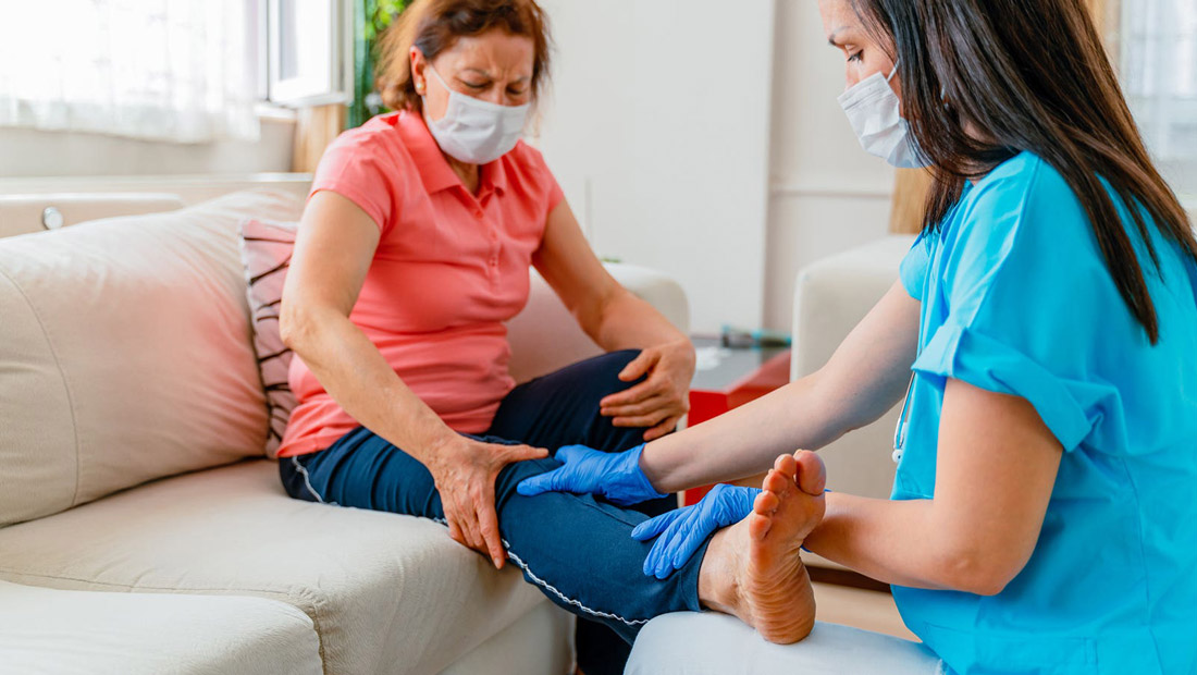
Blog

Thermodynamics of correlated electrons in a magnetic field

Thermodynamics of correlated electrons in a magnetic field

20:01 11 agosto in Artículos por Website
0


Interacting gap structure

In Fig. 1, we show the electron density 〈n〉 vs. chemical potential μ at different field strengths for U/t = 0–8. In Fig. 1a we observe an electron density plateau where there are energy gaps between magnetic Bloch bands, \(\langle n\rangle =2B\nu /{{{\Phi }}}_{0},\nu \in {\mathbb{Z}}\). As U increases in Fig. 1b–e, these plateaus are weakened and pushed outward in chemical potential, but inflections of the 〈n〉 vs. μ curves are still visible at the same density values, indicating that degeneracy of Landau levels is not modified by U. Since we are at relatively high temperature, only the most prominent band gaps (with Chern number C = ±1) 〈n〉 = 2B0 remain visible at larger U values. Additionally, at half filling, as U increases, a Mott gap appears and widens for all values of magnetic field. In Fig. 1d, e, for U/t ≥ 6, when the Mott gap is well-defined, it decreases monotonically as the magnetic field increases, consistent with previous exact diagonalization results24. The same trend can be seen in a “correlated Hofstadter butterfly” plot, as shown in Supplementary Fig. S1 and described in Supplementary Note 2. We will discuss later, and in more detail, the behavior of the Mott gap.

Fig. 1: Electron density vs. chemical potential.
Thermodynamics of correlated electrons in a magnetic field

Electron density 〈n〉 vs. chemical potential μ a in the non-interacting system, and be with Hubbard U/t = 2–8. Curves with the same color have the same magnetic field strength Φ/Φ0 across all panels. Each curve is plotted with an offset 2B0 in order to improve visibility of inflection points. Error bars, corresponding to ±1 standard error of the mean, estimated by jackknife resampling, are smaller than the size of data points. All plots have inverse temperature β = 4/t.

It is instructive to plot our data as Wannier diagrams44, i.e., color intensity plots of charge compressibility χ = ∂〈n〉/∂μ as a function of electron density 〈n〉 and magnetic field strength B. Charge compressibility, or thermodynamic density of states, is directly measurable in experiments9,13. In a non-interacting system, at zero temperature, charge compressibility is equivalent to the single-particle density of states. We measure charge compressibility in DQMC simulations as

$$\chi =\frac{\beta }{N}\mathop{\sum}\limits_{ij}[\langle {n}_{i}{n}_{j}\rangle -\langle {n}_{i}\rangle \langle {n}_{j}\rangle ],$$

(1)

where ni = ni + ni. In Fig. 2, we show Wannier diagrams for U/t = 0–6. For all values of U, we observe local minima of χ (indicating incompresssible states) along straight lines satisfying the Diophantine equation

$$\frac{\langle n\rangle }{{n}_{0}}=r\left(\frac{{{\Phi }}}{{{{\Phi }}}_{0}}\right)+s,$$

(2)

where r and s are integers, and n0 = 2 is the electron density of the completely filled system. This is consistent with what we expect from the Hofstadter spectrum in the non-interacting system44. The most prominent incompressible state with r = 1, s = 0 remains clearly visible up to U/t = 8. Less prominent incompressible states with r = 2 and r = 3 persist to U/t = 4 and U/t = 2, respectively. These results show that the integer quantum Hall states for r ≤ 3, s = 0 have no weak coupling instabilities with respect to Hubbard repulsion; the r = 1, s = 0 state remains stable up to large U. At half filling, the vertical compressibility minima indicative of the Mott gap becomes visible for U/t 4. Thus, we argue that the gross structure of magnetic Bloch bands and band gaps determined by the non-interacting Hofstadter spectrum is preserved in the presence of U, with the Mott gap at half-filling when U/t 4 superimposed as an additional feature. Due to the sign problem, our DQMC simulations are restricted to relatively high temperature βt ≤ 5, so we cannot resolve conclusively how much U changes the fine structure of the Hofstadter spectrum.

Fig. 2: Wannier diagrams.
figure 2

Wannier diagrams a in the non-interacting system and bd with Hubbard U/t = 2–6. Gray regions in bd are parameter regions where we don’t have simulation data. All plots have inverse temperature β = 5/t. Magnetic field strength is displayed as Φ/Φ0, and electron density is shown as 〈n〉/n0, where n0 is the electron density of a completely filled system, which in our case is 2. The system is particle-hole symmetric, so only the range 〈n〉/n0 [0, 0.5] is shown. Dotted cyan lines indicate where we expect local minima of charge compressibility to occur from the non-interacting model.

Fermion sign

An important quantity in QMC simulations of interacting fermions is the fermion sign. The Hubbard-Hofstadter model is sign-problem-free at half filling on a bipartite lattice. But the fermion sign problem45 fundamentally prevents us from obtaining high quality simulation data at low temperatures and away from half filling. Thus, any insight into factors affecting the severity of the sign problem is valuable. Since the fermion sign problem is NP-hard46, we do not expect a general solution to the fermion sign problem to exist. Nevertheless, as the sign problem is representation-dependent, it is possible to reduce or completely remove the sign problem for specific classes of non-generic Hamiltonians47.

In this work, we find a correlation between the fermion sign and the charge compressibility. In Fig. 3, we show the fermion sign 〈s〉 and charge compressibility χ, both plotted against 〈n〉, for one representative set of parameters. Local minima of charge compressibility in this interacting system exactly correspond to local maxima of the fermion sign. At these local maxima, the fermion sign may be an order of magnitude improved over its value at other electron densities and that of the standard zero-field Hubbard model. For an extended figure demonstrating that this correspondence is general across our parameter space and not a finite size artifact, see Supplementary Fig. S2 and Supplementary Note 3. Our results may mean that although the Hubbard model, in general, suffers from a sign problem, it is possible to obtain good results when we are precisely located on an integer quantum Hall plateau. Since similar sign-compressibility correspondence has been reported30,48,49,50, it appears that the improvement of fermion sign in insulating phases is quite general, consistent with our intuition that fermionic statistics become less important in localized states. Our results also relate to recent work51,52,53 suggesting that the fermion sign is not merely a coincidental barrier to accessing low-temperature physics, but may be reflective of intrinsic physics of model Hamiltonians.

Fig. 3: Fermion sign—charge compressibility correspondence.
figure 3

a Charge compressibility χ = ∂〈n〉/∂μ and b fermion sign 〈s〉 plotted against electron density 〈n〉 at magnetic field strength Φ/Φ0 = 12/64, inverse temperature β = 6/t and Hubbard interaction U/t = 4. This system is particle-hole symmetric, so we only plot the density range 〈n〉  [0, 1]. Dashed lines indicate electron densities at which χ reaches local minina and 〈s〉 reaches local maxima. Error bars, corresponding to ±1 standard error of the mean, estimated by jackknife resampling, are smaller than the size of data points.

Half-filling

Finally, we focus on half filling, where we believe interesting interplay between Hofstadter physics and Hubbard physics occurs. In the absence of a magnetic field, the ground state of the half-filled Hubbard model is an AFMI at any nonzero value of U, i.e., (Uc = 0)29,30, due to perfect nesting of the Fermi surface and a logarithmically divergent single-particle density of states. In the limit of strong interactions Ut, the half-filled Hubbard model maps to the Heisenberg model with antiferromagnetic nearest neighbor spin exchange energy J = 4t2/U54.

In the presence of an orbital magnetic field, the non-interacting density of states at half filling is modified significantly. As can be seen in Fig. 2a, the density of states/charge compressibility does not change monotonically with field, but instead shows prominent minima at Φ/Φ0 = p/q, where p and q are co-prime and q is even, corresponding to a non-interacting ground state with q inequivalent Dirac cones37. The large-field limit corresponds to the π-flux model, in which a semimetal–AFMI transition occurs at Uc ≈ 5.6t. As the orbital magnetic field significantly changes the non-interacting density of states at half filling, we expect that critical Uc should exhibit B field dependence. It would be interesting to investigate if Uc changes monotonically with B, or if it exhibits non-monotonicity commensurate with the oscillatory behavior of the density of states. We defer the mapping of this UB phase diagram to future work.

For the remainder of this section, we focus on the parameter region U/t [6, 10]. Here, the system is safely an AFMI at all field strengths. We examine the evolution of local magnetic moment \(\langle {m}_{z}^{2}\rangle\), antiferromagnetic structure factor S(π, π) and specific heat cv = ∂〈E〉/∂T with magnetic field strength, and see that these thermodynamic quantities all consistently show that a strong orbital magnetic field tends to modify the AFMI by delocalizing electrons and thereby reducing the effect of U on the low-energy properties of the Mott insulating phase. For finite-size analysis of thermodynamic observables at half filling, see Supplementary Fig. S3 and Supplementary Note 3.

In Fig. 4, we show the temperature and field dependence of the local moment. The local moment or sublattice magnetization

$$\langle {m}_{z}^{2}\rangle =\frac{1}{N}\mathop{\sum}\limits_{i}\langle {({n}_{i\uparrow }-{n}_{i\downarrow })}^{2}\rangle$$

(3)

measures the degree of spin localization. It is 0.5 in the non-interacting system and approaches 1 in the U/t →  limit. In the zero-field Hubbard model, \(\langle {m}_{z}^{2}\rangle\) has features at T ~ U associated with the formation of local moments, and at T ~ J, associated with short- or long-range ordering of local moments36,55. We see that at fixed U, increasing magnetic field strength reduces the local moment monotonically at all temperatures, with the effect largest below temperatures T ~ J. The zero-field and π-flux limit of local moment data are consistent with previous work43.

Fig. 4: Evolution of local moment and magnetic structure factor in the half-filled Hubbard–Hofstadter model.
figure 4

Temperature and field dependence of local moment \(\langle {m}_{z}^{2}\rangle\) at half filling. Insets display the field dependence of magnetic structure factor S(π, π) at βt = 16 for magnetic field strength Φ/Φ0 [0, 0.5]. ac Correspond to Hubbard interaction strength U/t = 6–10, respectively. Curves with the same color and marker type have the same magnetic field strength across all panels. Error bars, corresponding to ±1 standard error of the mean, estimated by jackknife resampling, are smaller than the size of data points.

The magnetic structure factor is the Fourier transform of the real-space spin–spin correlation function

$$S({{{{{{{\bf{Q}}}}}}}})=\frac{1}{N}\mathop{\sum}\limits_{ij}{{{{{\rm{e}}}}}}^{{{{{{{{\rm{i}}}}}}}}{{{{{{{\bf{Q}}}}}}}}\cdot ({{{{{{{{\bf{R}}}}}}}}}_{i}-{{{{{{{{\bf{R}}}}}}}}}_{j})}\langle ({n}_{i\uparrow }-{n}_{i\downarrow })({n}_{j\uparrow }-{n}_{j\downarrow })\rangle .$$

(4)

When the system has long-range antiferromagnetic order, the structure factor is strongly peaked at the ordering wave vector Q = (π, π), with peak height scaling linearly with lattice size36,56. In our simulations, we find that at all B and U values, the magnetic structure factor is sharply peaked at (π, π), consistent with the system being in the AFMI phase. Insets to Fig. 4 show that at all U, the magnetic field monotonically reduces S(π, π), indicating that the magnetic field reduces the AFMI ordering tendencies.

Figure 5 shows the evolution of the low temperature peak of cv with magnetic field and Hubbard U. We calculate cv numerically by measuring energy as a function of temperature 〈E(T)〉 and taking the finite difference Δ〈E〉/ΔT. In the zero-field half-filled Hubbard model, at large U, the specific heat has a “two peak” structure, with a broad high temperature peak at T ~ U associated with charge fluctuations and and a narrow low temperature peak at T ~ J associated with spin fluctuations55,57. When a magnetic field is turned on, as shown in Fig. 5b, c, U is large enough that the two peaks remain well-separated. The high temperature peak doesn’t move, while the low temperature peak shifts to higher temperatures. In Fig. 5a, the two peaks are initially well-separated at low fields, but at Φ/Φ0 1/4, the low temperature peak shifts upwards and merges with the high-temperature peak, complicating our interpretation. This is likely due to U/t = 6 being low enough for the system to not simply map to the Heisenberg model, and for the system to be close to the AFMI phase transition at π-flux.

Fig. 5: Evolution of specific heat and kinetic energy in the half-filled Hubbard–Hofstadter model.
figure 5

Temperature and field dependence of specific heat cv at half filling. Insets display the field dependence of kinetic energy 〈K〉 at βt = 16 for magnetic field strength Φ/Φ0 [0, 0.5]. ac Correspond to Hubbard interaction strength U/t = 6–10, respectively. Values of J = 4t2/U are also indicated for each U. Curves with the same color and marker type have the same magnetic field strength across all panels. Error bars denote ±1 standard error of the mean, estimated by jackknife resampling.

Since the low temperature peak in specific heat is associated with the spin exchange energy J, we are tempted to say that the orbital magnetic field increases J. However, this interpretation may be overly naive. We believe the more accurate statement is that the orbital magnetic field tends to delocalize electrons, and thus, effectively lower the influence of U on low energy properties of the system. Insets to Fig. 5 show that a magnetic field increases (in magnitude) kinetic energy in the insulating phase, which supports this interpretation. This runs contrary to our usual intuition that an orbital magnetic field localizes electrons by winding them up into Landau orbits. However, here our starting point is a correlated insulator, rather than free electrons (or a Fermi liquid). Our results in Figs. 45, along with the decreasing width of the Mott gap in Fig. 1d, e, suggest that in the AFMI phase, the orbital magnetic field tends to delocalize electrons, increase kinetic energy, and lower the effective influence of U. We observe that the influence of magnetic field is suppressed as U increases. As U/t → , the influence from the B field will diminish and become negligible, since in the atomic limit, no hopping exists, and the orbital magnetic field cannot have an influence on the system.


Source link